Dual vector spaces pop up in relativity and quantum mechanics. Each time I’ve read about them, I’ve felt like I “got it” just enough to do the calculations. The details of how you go about constructing these things were a bit muddy, though. So, on the pretext that the best way to understand is to explain, I’ll try to outline the bare bones ideas below. Hopefully, I’ll keep fleshing this out with more interesting stuff as time rolls on.
I’ll use an unconventional notation for this post. That’s because the conventional notation is suggestive of what you know by the end of the argument, but I don’t want to begin at the end! The conventional notation (bra-ket in quantum mechanics or upper and lower indices in relativity) makes a lot of sense to the initiated, but is confusing when laying out the groundwork for the first time. After we get that groundwork down, I’ll backtrack and review the ideas using standard notation.
Disclaimer: I do not vouch for the accuracy of what appears below. This is just me, trying to define the things we use in physics in a way that I can understand. I just hope I don’t mutilate it too badly. Also, to any knowledgeable readers who wish to leave some feedback, I’d be grateful.
Let 
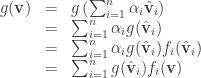
A one form 

where 

where 
and 
Define addition of one forms by
![\left[ f+g \right] \left( \mathbf{v} \right) = f \left( \mathbf{v} \right) + g \left( \mathbf{v} \right)](https://s0.wp.com/latex.php?latex=%5Cleft%5B+f%2Bg+%5Cright%5D+%5Cleft%28+%5Cmathbf%7Bv%7D+%5Cright%29+%3D+f+%5Cleft%28+%5Cmathbf%7Bv%7D+%5Cright%29+%2B+g+%5Cleft%28+%5Cmathbf%7Bv%7D+%5Cright%29&bg=ffffff&fg=333333&s=0&c=20201002)
Addition of one forms is then commutative and associative, because addition of real numbers has those properties.
Define scalar multiplication of one forms in the obvious way:
![\left[ \alpha f \right] \left( \mathbf{v} \right) = \alpha * f \left( \mathbf{v} \right)](https://s0.wp.com/latex.php?latex=%5Cleft%5B+%5Calpha+f+%5Cright%5D+%5Cleft%28+%5Cmathbf%7Bv%7D+%5Cright%29+%3D+%5Calpha+%2A+f+%5Cleft%28+%5Cmathbf%7Bv%7D+%5Cright%29&bg=ffffff&fg=333333&s=0&c=20201002)
Now note that

is linear, and therefore a one form. Zero is the additive identity for the field, so 
Each one form has a unique inverse

All this means that the one forms themselves form a vector space. (If you’re worried about some vector space prerequisite I didn’t mention, such as existence of a multiplicative identity, you can check for yourself that it’s in there. I’m not tricking you.)
Now we want to know the dimension of the space of one forms. We suspect that it’s the same as the dimension of
Due to linearity, the action of a one form on any vector in 

For each basis vector,

The above equation is defining the action of the one form 

I claim that these
Clearly they are independent, because assuming they are dependent gives, for some set of not-all-zero coefficients 

which is a contradiction, because it was assumed that not all the coefficients were zero. The last equality in the above equation comes from 
The 
which implies

This means the
Here comes the part that tricked me before. We’re going to change our definition of
The change is that before, the basis vector 

This is a bit subtle. We’re changing the original vector space from just a nice little vector space sitting all alone by its logical self, into being the space of all linear transformations on the one forms. We already know that the set of all linear transformations on the one forms is indeed a vector space, because all the arguments we used before when showing that the one forms are a vector space can trivially cascade down to this redefinition of
The problem is that we’re redefining
The solution to this cute little quandary is that really what we want to do is redefine both vector spaces at the same time. We want to define them so that each one is the set of linear, scalar-valued functions of the other. We began this discourse with an asymmetry between the vectors and the one forms. Now I’m saying we should abolish that asymmetry. Really, we should have skipped all the business with the original vector space from the beginning. We should have started off by defining two vector spaces, 
The reason I didn’t start out that way was that I thought it would be too confusing. I thought the definition would sound circular. In fact it’s not. It’s completely reasonable, but only once you know the sort of facts we worked so hard to find out. It can only work because the one forms make a vector space of the same dimension as the original vector space.
So let’s do it properly, from the beginning, in a different notation.
Let 

The trick is in seeing that this makes any sense – that such a thing is possible. That’s what all the nonsense above was about. It says that by starting with a vector space, either
Finally, we’ll discuss notation. In quantum mechanics, elements of

while the elements of

The notation for one acting on the other (it doesn’t matter which acts on which) is written

In relativity, the elements of

where 


The elements of

One vector acting on a covector (or covector acting on a vector) is written

You can take the first step in that equation by the definition of the basis vectors acting on each other. The second step is a sum of the
Finally, you may also be familiar with the notation in which elements of
